Rigid Body Rotation
09 Sep 2020
Introduction
Have you ever wondered why you can’t seem to rotate a tennis racket head-over-handle? If you do, it won’t do it in a stable manner, it will flip along other directions too. This is a demonstration of the intermediate axis theorem (also referred to as the tennis racket theorem or the Dzhanibekov effect). It is a feature of Euler’s equations which govern rigid body rotation. His equations are first-order ordinary differential equations (ODEs), but they are by no means trivial to solve since they are coupled and non-linear.
Rigid bodies and Euler’s equations have been studied in detail for at least the last 200 years and exact solutions are known, although they involve elliptic functions. An easier way to visualize the problem was coined by Poinsot, known as Poinsot’s construction. Instead of solving Euler’s equations, Poinsot enforced conservation of energy and angular momentum as constraints on the solutions, and visualized the solution paths as the intersection between surfaces.
I claim however that to understand the intermediate axis theorem, one does not need to directly solve Euler’s equations, or even enforce conservation constraints. With some manipulation, all of the dynamical features of rigid body rotation can be visualized graphically.
Euler’s Equations
To analyze the rotational dynamics of rigid bodies, I start with Euler’s equations in three dimensions (in the absence of applied torque),
\[I\frac{d \vec \omega}{dt} +\vec\omega\times(I\vec\omega)= 0\,,\tag{1}\]where $I$ is the $3\times3$ inertia tensor and $\vec\omega$ is the angular velocity vector of the rigid body. Equation (1) is derived from Newton’s second law, but adapted into the body-fixed reference frame. The reason for this is that it ensures that the inertia tensor of the body is not changing with time. First I will substitute the body-fixed angular momentum $\vec L=I\vec\omega$ to obtain
\[\frac{d \vec L}{dt} =\vec L\times(I^{-1}\vec L)\,.\tag{2}\]I will then choose a Cartesian basis $(x,y,z)$ that is aligned with the angular momentum components such that the inertia tensor can be diagonalized as
\[I =\left(\def\arraystretch{1.1}{\begin{array}{ccc} I_x & 0 & 0\\ 0 & I_y & 0 \\ 0 & 0 & I_z\end{array} }\right)\,.\tag{3}\]At this point, I am motivated to try to reduce this system to a two dimensional one, because three dimensions is just too many. To do this, I will represent this system of equations in terms of spherical coordinate variables $(r,\phi,\theta)$. In terms of these variables, the angular momentum vector can be expressed as
\[\vec L =L\left[\cos(\phi)\sin(\theta)\hat x + \sin(\phi)\sin(\theta)\hat y + \cos(\theta)\hat z\right]\,.\]I can then substitute this into Equation (2) along with Equation (3) to obtain
\[\begin{align} \frac{1}{L^2}\frac{d \vec L}{dt}& =\;\frac{(I_y-I_z)}{I_y I_z}\sin (\theta ) \cos (\theta ) \sin (\phi )\hat x\nonumber\\& +\frac{(I_z-I_x)}{I_x I_z}\sin (\theta ) \cos (\theta ) \cos (\phi )\hat y\\& +\frac{(I_x-I_y)}{I_x I_y}\sin ^2(\theta ) \sin(\phi ) \cos (\phi )\hat z\,. \end{align}\]This Cartesian vector can then be expressed in terms of the spherical coordinate unit vectors $(\hat r,\hat\phi,\hat\theta)$ by transforming it with the Cartesian-to-spherical transformation matrix,
\[T_{x\rightarrow r}=\left(\def\arraystretch{1.5} \begin{array}{ccc} \sin (\theta ) \cos (\phi ) & \sin (\theta ) \sin (\phi ) & \cos (\theta ) \\ -\sin (\phi ) & \cos (\phi ) & 0 \\ \cos (\theta ) \cos (\phi ) & \cos (\theta ) \sin (\phi ) & -\sin (\theta ) \\ \end{array}\right)\,,\]which results in
\[\begin{align} \frac{1}{L^2}\frac{d \vec L}{dt} =&\frac{\left[I_x I_z+I_y I_z-2 I_x I_y+I_z (I_y-I_x) \cos (2 \phi )\right]\sin (2\theta )}{4I_x I_y I_z }\hat\phi+\frac{(I_y-I_x) \sin (\phi) \cos (\phi )\sin (\theta ) }{I_x I_y}\hat\theta\,.\tag{4} \end{align}\]Notice that the $d \vec L/dt$ vector has no component along the $r$-direction, as should be expected given that the magnitude of $\vec L$ should not change due to the conservation of angular momentum. Just by converting Euler’s equations to spherical coordinates, we have just proven that his equations obey this crucial conservation law. The system has thus been successfully reduced to a two dimensional problem.
The Intermediate Axis Theorem Demonstrated
The result obtained in Equation (4) can now be plotted in a phase diagram, a plot that shows the direction of the vector field $d\vec L/dt$ as a function of $(\phi,\theta)$. Keeping in mind that vector derivatives are scaled differently in spherical coordinates compared to Cartesian ones,
\[\frac{d\vec L}{dt}=\left(\frac{dL}{dt}\right)\hat r + \left(\frac{d\phi}{dt}\right)L\sin(\theta)\hat\phi + \left(\frac{d\theta}{dt}\right)L\hat\theta \,,\]I will pick out just $d\phi/dt$ and $d\theta/dt$ for the plot. To ensure there is an intermediate axis, it is assumed that $I_x<I_y<I_z$. This defines the $y$-axis as the intermediate axis.
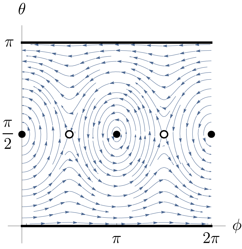
The above figure is a phase diagram for rotating rigid bodies. Black dots and lines represent fixed points called centers. When the system starts near these points, the vector $\vec L$ will “orbit” around these points indefinitely, which is known as precession in rotational dynamics. The open circles represent unstable fixed points, where solution curves are repelled from being near for too long. I used Wolfram Mathematica to make this plot, and took $I_x=1$, $I_y=1.5$, $I_z=2$.
To better understand the question at hand though, Equation (4) can be converted to be in terms of the angular velocity $\vec\omega$. The vector field $d\vec L/dt$ needs only to be rescaled by the inverse of the inertia tensor (after it is converted back to Cartesian coordinates),
\[\frac{d \vec \omega}{dt} =I^{-1}\frac{d \vec L}{dt}\,.\]This allows for the projection of the vector field onto the Poinsot ellipsoid, the surface that the angular velocity vector $\vec\omega$ is constrained to move on, demonstrated below.
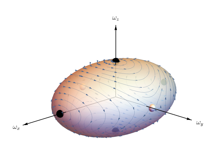
This is now a phase diagram for rigid body rotation in three dimensional angular velocity space. Black dots represent the center fixed points, while white dots represent the unstable fixed points on the intermediate axis. Generated with Wolfram Mathematica, with $I_x=1$, $I_y=1.5$, $I_z=2$.
So what happens when you try to flip a tennis racket? If you calculate the inertia tensor for the racket, you will find that trying to flip the head of the racket over the handle is equivalent to rotating a rigid body around the unstable intermediate axis. You could, in theory, rotate it on this axis, but it would quickly decay under any small perturbation, like trying to balance a ball on a horse’s saddle. The racket will then settle onto a path that passes close to the unstable axis, but ultimately precesses around one of the stable axes. You can visually follow the path of precession using the above figure, and such trajectories are called polhodes in the literature. Since the path does indeed pass close to the unstable axis anyway, it may appear to rotate around it briefly, but it will continue its precession around to the opposite axis, resulting in what looks like a “flip”.